Cover
The cover of plants is the amount of ground surface beneath plant materials (basal, foliar, live, dead and/or total) or other objects (litter, rocks, etc.). Because different methods and decision rules can lead to very different cover numbers for the same vegetation, it is critical to be clear which cover technique is used and to carefully follow the measurement rules. Canopy cover, foliar cover, ground cover, and basal cover are defined in the glossary, Appendix M. Species can later be grouped by life form or functional groups.
Cover characteristics can be determined in conjunction with frequency sampling by recording “hits” at marked points on a tape, or corners of a frequency frame or grid. However, this sampling intensity may not provide an adequate measure of basal cover of individual plant species, and conclusions about basal cover should not be made without a large enough sample size to make the sampling statistically valid. The Ground Cover and Canopy Cover Measurements side bar further describes a procedure for obtaining cover data.
Canopy Cover
Canopy cover is the percent of ground covered by a vertical projection of the outermost perimeter of the natural spread of foliage, including small openings. Because of overlapping canopies, it may exceed 100 percent for the community if data are collected by plant species or functional group. This is often collected using line intercept (BLM 1999a) and can also be collected with grid plots or Daubenmire frames (BLM 1999a). Canopy cover provides many useful interpretations, especially for shrubs. For example, sagebrush line intercept cover has often been used to describe habitat values and make management recommendations (Rassmussen et al. 2001). Canopy cover of herbaceous species varies greatly among seasons and years, much more than basal ground cover.
 Figure 26. Cover of USDI-BLM (1999a).
Ground Cover and Canopy Cover Measurements
Foliar cover is the area of ground covered by the vertical projection of the aerial parts of plants. Canopy cover is similar but does not exclude small voids, or it estimates a polygon around the outer parts of the canopy. Ground cover is the area or percent of ground surface occupied by the basal portion of individual plants or by bare ground, rock, litter and soil biotic crusts (where identifiable). See glossary for precise definitions. Basal cover or ground cover of live vegetation can quickly be obtained, along with frequency information, by observing cover at specific points along the transect and/or quadrat frame.
Common methods used to measure cover are line intercept (canopy or basal cover) and point intercept (foliar or ground cover). When using line or point intercept, it is important to observe enough line length or points to get a reliable estimate. Using five transects usually reduces the standard deviation. It is important to strictly follow the set of rules used among individuals from monitoring period to monitoring period (Elzinga et al. 1998). Foliar or canopy cover is often less useful for herbaceous plants (especially bunch grasses) than basal cover because the aerial parts of the plants vary with season, year and grazing use.
In some instances, species groups, e.g., grasses, forbs or shrubs, can be lumped into functional groups. The applicability of grouping by life form depends on the objectives. Also, species data can always be lumped for analysis, but lumped field data cannot later be split. For an additional discussion of cover monitoring see Sampling Vegetation Attributes (BLM 1999a).
 Figure 27. Canopy cover is often measured
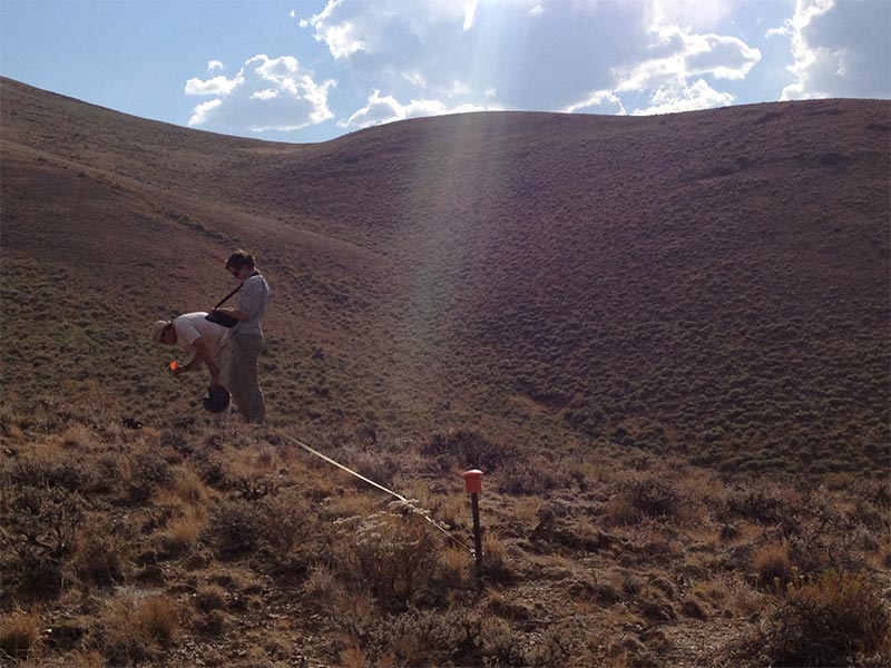 with a stretched measuring tape
 using either line intercept or line point intercept,
 which is often used for foliar, basal or ground cover.
Foliar Cover
Foliar cover is the amount of leaves and stems that could intercept raindrops or provide shade from a vertical sun. Foliar cover is less than canopy cover because it does not include gaps within the canopy. This is measured with line point intercept or any dimensionless point tool such as a pin drop, laser pointer or other sighting tool. It is being used extensively by the BLM in Assessment, Inventory and Monitoring (AIM) and by NRCS in National Resources Inventory (NRI).
Basal Cover
Basal cover is the area of the ground surface covered by the basal part of plants. For trend comparisons in herbaceous plant communities, perennial grass basal cover is generally considered to be the most stable. It does not vary as much due to climatic fluctuations or current year grazing (BLM 1999a).
Ground Cover
Ground over is most often referred to as the percentage of ground surface covered by plants, litter, microbiotic crust, rocks and gravel. Ground cover is an important soil-surface attribute (BLM 1999a; Herrick et al. 2005a and b). It and foliar cover have been most often correlated to rangeland hydrologic function. Change in ground cover is an important aspect of trend. It is very useful for establishing planning objectives. It is also used to determine if favorable or unfavorable conditions exist for germination and establishment of new plants, and to assess nutrient cycling.
Community-Type Transects
The proportion of the area occupied by various community types can be used as the unit of measure (e.g. Winward 2000) in riparian areas, where the number of species is often greater than on uplands, and where many plant species are rhizomatous. Cross-valley transect data are collected along five parallel transects that cross the riparian area perpendicular to the long axis of the riparian area (e.g., valley) (Winward 2000). They are used where objectives relate to vegetation away from the stream edge.
More commonly, community types or dominance types are monitored along the greenline (Winward 2000; Burton et al. 2011; Perryman et al. 2017) or streamside (Perryman et al. 2006). Stabilizing plants are needed where they can buffer the forces of flowing water and influence erosion and sediment deposition. The greenline is the first line of perennial vegetation on or near the low water edge. Most often it occurs at or slightly below the bankfull stage. For more details about these methods. See Winward (2000) or Burton et al. (2011). Similar data without the species identified can be collected by life form along the water’s edge (see the Ranchers’ Monitoring Guide, (Perryman et al. 2006) or greenline (Perryman et al. 2018).
Winward (2000) presents guidelines for setting long-term objectives by riparian capability groups. Objectives for designated monitoring areas should also be based on an understanding of stream dynamics and the processes of stream recovery after channel incision or other problems. Rosgen (1996) stream classification or a geomorphic analysis and PFC assessment (Prichard et al. 1998; Dickard et al. 2015) can help locate stream reaches responsive to management and help in setting objectives. In areas where community types are not well classified or understood by the observers, vegetation can also be observed and recorded by noting the dominant species in plots or in patches of similar vegetation (e.g. MIM Burton et al. 2011).
Greenline transects sometimes measure revegetation on point bars, but will not where the greenline is well above the revegetating point bar. To capture vegetation trends early in the recovery process, the point bar may be a place of focus. However, point bars are also places of natural sediment deposition, and colonizers may be washed away or buried. Therefore, point bar measurements, although often interesting and useful, can also be misleading if not interpreted in light of intervening flow records.
Greenline-to-Greenline Width
The distance across a creek from the greenline on one side to the greenline on the other side is another way to assess point bar revegetation and the narrowing of streams (Burton et al. 2011). Very often, problematic riparian grazing management weakens streambanks and leads to or perpetuates over-wide channels that reflect poor fish habitat and water quality. When grazing management that enables riparian recovery of functions and values (Wyman et al. 2006; Swanson et al. 2015) is implemented, greenline-to-greenline width is often the most notable indicator of recovery.
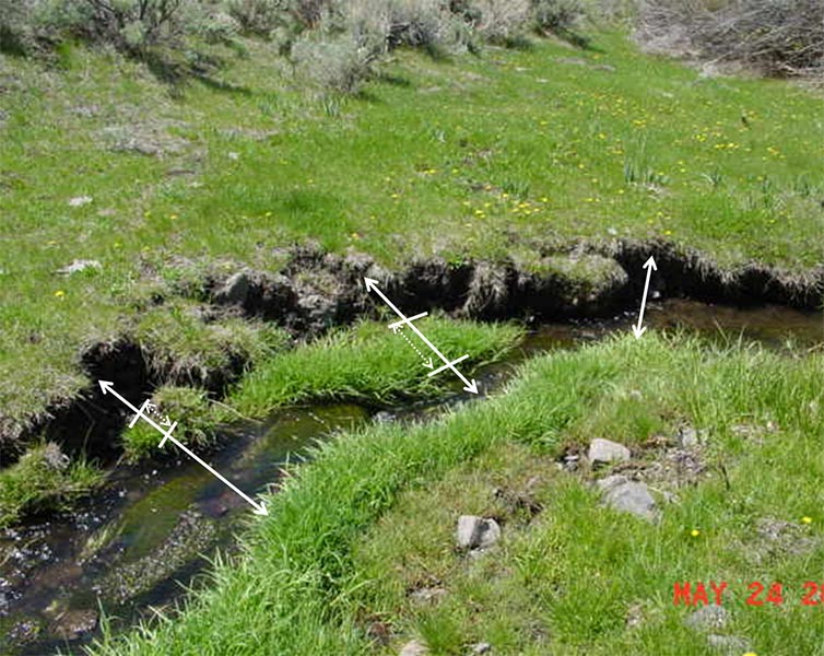 Figure 28. Many streams recovering after a change in riparian grazing management narrow in their greenline-to-greenline width. (Burton et al. 2011).
Riparian Shrubs
Winward (2000) and Burton et al. (2011) also describe methods for monitoring woody species abundance, regeneration and height. Both methods may require some practice in order to collect consistent data (Coles-Ritchie et al. 2004). Riparian shrubs can also be monitored with line intersect or air photos for canopy cover, which can be augmented with height for measurements for canopy volume. Doing this requires careful consideration to match methods with site potential and objectives. Where wildlife habitat considerations warrant, a robel pole can be used to measure visual obstruction at various heights (BLM 1999a).
Streambank Stability
Burton et al. (2011) describe streambank stability for nondepositional streambanks as a combination of cover and stability, versus uncovered and mass wasting. Streambanks are covered and stable if they are covered with perennial vegetation, cobble-size or larger rock, or anchored wood, and they do not have indications of erosion, breakdown, shearing or trampling that expose plant roots. Change in streambank stability may reflect incision, healing or accumulated damage from use impacts such as streambank alteration. Failure to improve may otherwise reflect nonfunctional conditions, such as concentrated stream energy after channel incision or other impacts that are not related to grazing management (e.g. altered flow regime, OHV use, etc.).
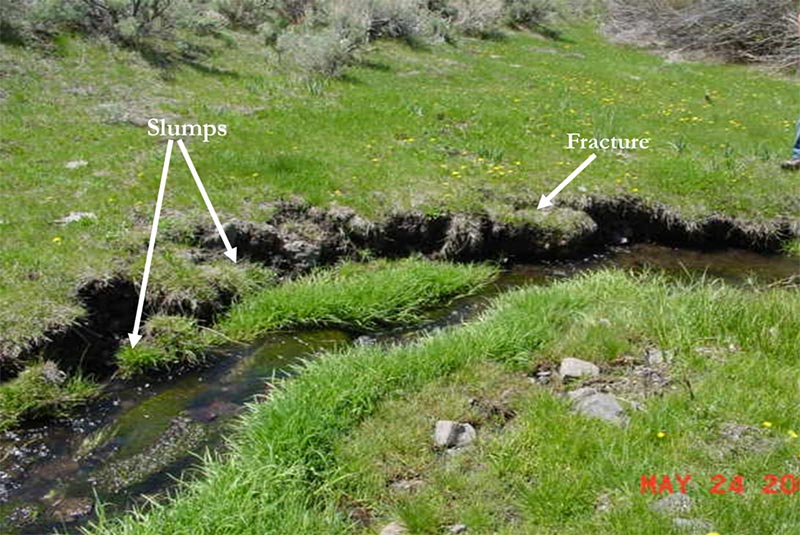 Figure 29. On some streams, the instability of banks with slumping or fractures indicate recent incision or weakened riparian root systems (Burton et al. 2011).
Stream Channel Attributes
Stream channel morphology provides habitat features important to fish for hiding or foraging, and also affects channel stability and water quality. Land managers sometimes monitor stream channel characteristics (e.g., width/depth ratio, depth, or pool quality) for improvement or degradation from management actions. However, the driver of channel attributes is usually riparian functionality (Dickard et al. 2015) especially greenline vegetation. Monitoring vegetation with MIM (Burton et al. 2011) provides more timely and sensitive data for detecting change in relation to management. Also, it is important to recognize that desired channel attributes differ among species needing habitat. Some desert spring fish and amphibians evolved with high levels of disturbance and may require different habitat characteristics than commonly associated with good habitat for others (Kodric-Brown and Brown 2007).
Stream Survey
The General Aquatic Wildlife Survey (GAWS) (FS 1985) and BLM Stream Survey (Elko BLM 2002) have provided valuable baseline information since the late 1970s and have often guided management changes. These surveys contain photographs, in addition to stream and fish habitat measurements and riparian observations related to optimal conditions for cold-water fish (but not in relation to site potential). Stream survey scores generally do not make useful objectives because they combine numerous variables representing a variety of factors into one index. Index improvement is only partially tied to specific management actions or plans. An index may not change while two or more of the index’s components change measurably, some increasing and others declining. Combining understanding of process developed through riparian proper functioning condition assessment with the quantification from stream surveys leads to greater utility from both data sets. Multiple indicator monitoring (MIM) uses many more independent plots and provides a much more sensitive measure of change through time at a location (Burton et al. 2011).
Water Quality
BLM and the FS comply with the Clean Water Act (and in places, the Safe Drinking Water Act) and other federal laws and executive orders, that require attainment and maintenance of water quality standards. Protocols for monitoring water quality attributes, such as various plant nutrients, temperature, fecal coliform, etc., have been developed and are used by the Nevada Division of Environmental Protection (NDEP) and other agencies. The NDEP has signed a memorandum of understanding with the BLM and FS, addressing authorities and protocols for water quality monitoring. Water quality data should be interpreted carefully because it often does not reflect current or on-site management, but rather a combination of uncontrollable watershed and upstream factors, such as geology, climate, channel geomorphology and stream dynamics, etc.
Where there are water quality problems, it is best to determine the underlying causes and to manage and monitor accordingly. For example, streams that have poor water quality are often not functioning properly. Managing and monitoring for stabilizing riparian vegetation is usually the most effective way to address rangeland water quality problems unless they are caused by a discrete source of contaminants(Kozlowski et al. 2013; Swanson et al. 2017). Riparian vegetation improvements occur faster than improvements to stream channels, which occur quicker than changes in water quality but which also drive desired changes in water quality (Wyman et al. 2006).
The Nonpoint Source Management Program of the NDEP has worked with the Nevada Creeks and Communities Team to support the use of PFC (Dickard et al. 2015) grazing management practices and riparian habitat restoration (NDEP 2015). Riparian concepts are embraced throughout the 2015-2019 Nevada Nonpoint Source Management Plan.
Canopy Gap Intercept
Canopy gap intercept measurements provide information about the proportion of soil surface in large intercanopy gaps. Large gaps between plant canopies have the potential to facilitate wind erosion and invasive species establishment. As vegetation height increases, the gap size that allows wind erosion also increases. Canopy gap is measured along a line-intercept transect. For the National Resources Inventory Protocol – canopy occurs any time more than 50 percent of any 0.1 foot of tape edge intercepts live or dead perennial or annual plant material based on a vertical projection from canopy to ground. Canopy gap is an area along the tape edge that is absent of any plant canopy if the gap is 1.0 foot (30 cm) or greater in width (MacKinnon et al. 2011) . Perennial gaps can also be measured if all annuals are excluded as a gap disrupter. The length of each gap is calculated, and the sum of the lengths is divided by the transect length to obtain the proportion of soil surface in large intercanopy gaps. Number of gaps in various gap-size-length groups and distances between gaps are also useful. Appropriate gap size varies by ecological site, state and phase. The management interpretations differ widely among areas. Therefore, gap size should not be used independently of other vegetation measurements.
Plant Density
Plant density is the number of individuals of a species, or of each species, per unit area. Density measurements can be used to track population response to treatments, such as weed control, seeding establishment (or success through time), or enhancement strategies for key species. Density measurements may address an entire population with a total count, if small in size and area. Usually, density measurements track an area with a sampling protocol, using multiple quadrats or one or more belt transects. Population dynamics can be tracked by noting or counting by age or size classes of woody plants or perennials (Elzinga 1998; BLM 1999a; Winward 2000; Burton 2011). Density varies by ecological site, state, phase, plant size, and population size structure. The management interpretations differ widely among areas. Therefore, density should not be used independently of other vegetation measurements.
Vegetation Height
Vegetation height describes the vertical structure of vegetation, which can be used to characterize wildlife habitat, model fuels and estimate wind erosion. This method is a fast and unbiased way to measure vertical structure of vegetation. When used together with the proportion of the soil surface in large intercanopy gaps, it can be used to create three-dimensional models of vegetation structure. For the NRCS NRI and BLM AIM protocols, the height of a leaf, stem or seed head (nonstretched and living or dead) of woody and herbaceous plants within a 6-inch radius is recorded at selected points at fixed intervals along a transect. If vegetation is taller than 10 feet, a standard tape and clinometer method is used to estimate vegetation height.
Forb Abundance and Diversity
Forbs are valuable in the diets of many herbivores and often support pollinators. Forb diversity, or any species diversity, can be evaluated with a variety of species composition metrics (species list, cover, density, production, frequency) and evaluated using various diversity indices. However, all diversity is not equally useful (e.g. noxious weeds). Sage-grouse chicks depend on select protein-rich forbs for growth and development until fall when they switch to a diet of mostly sagebrush. The Habitat Assessment Framework (HAF) (Stiver et al. 2015) provides specific methods for monitoring forb abundance and diversity in sage-grouse habitats.
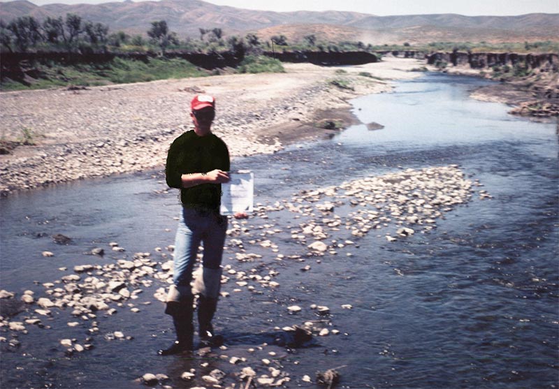 Figure 30. Many streams that do not meet water quality standards or that could meet water quality goals at a higher level have been impacted by loss of riparian functions.
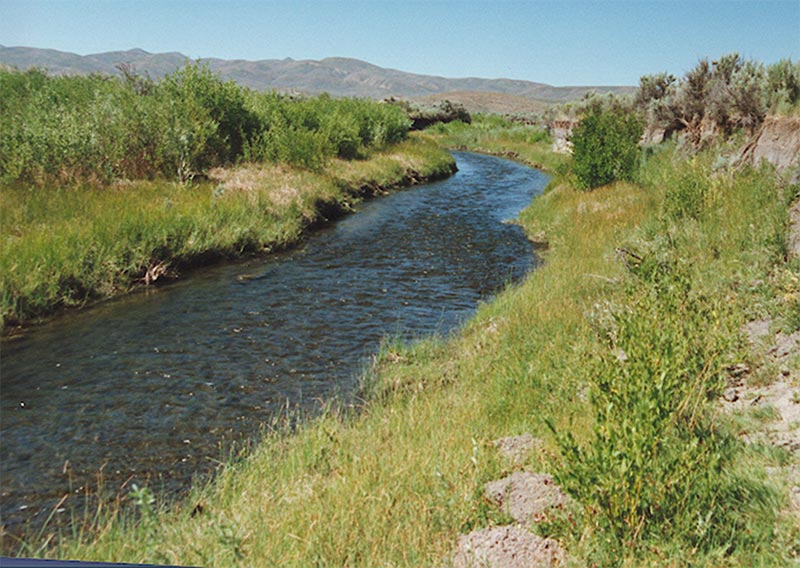 Regaining functions can recover water and aquatic habitat quality such as happened on Maggie Creek (Kozlowski et al. 2013).
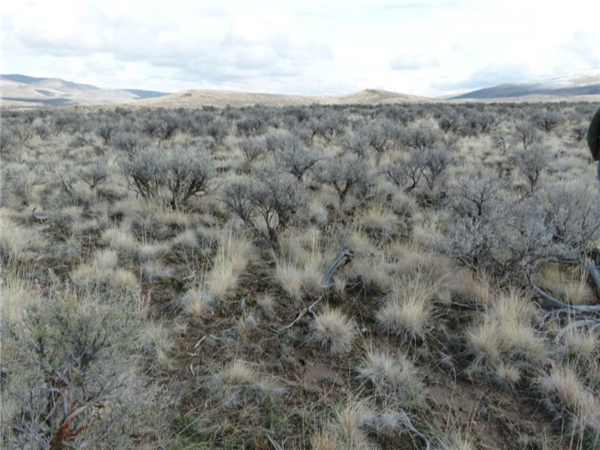
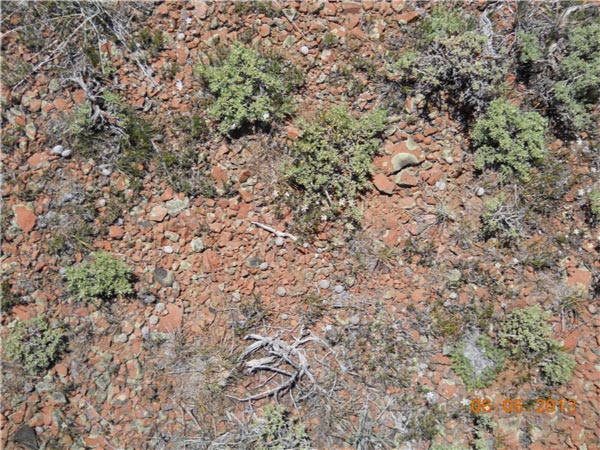
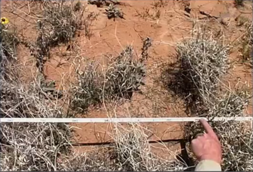 Figure 31. Canopy gap measurements provide indications of susceptibility to wind erosion and invasive species.
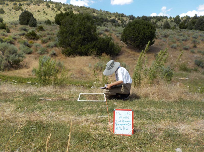 Figure 32. Measurements of forb density, species diversity, or forb cover often are taken in sage-grouse late brood rearing habitat where riparian soil moisture keeps protein-rich forbs green after upland forbs have dried out in the normally dry summers of the western and northern Great Basin.
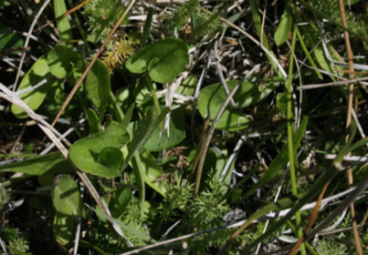 Figure 33. A diversity of riparian forbs provides a choice to sage-grouse chicks.
Section Summary
Long term monitoring tracks accomplishment of objectives to understand the appropriateness of management; therefore, there must be strong connection between the methods chosen and the SMART objectives. These objectives must be measured in appropriately selected key areas that reflect the opportunity for management to achieve the desired outcome. Long-term monitoring information is supported by, but not replaced by, short-term monitoring.