Introduction
Virtually every measurement of nature shows variation. Scientists have developed procedures for sampling and replication to improve their confidence that the data they collect provides a reliable estimate of the population sampled, and any change(s) (or lack thereof) in important attributes related to the implementation of management actions. Generally, using more samples with additional data points increases the ability to detect important differences for one or more attributes among populations and/or communities, or for the same population/community attribute across time. With enough data, one can detect differences so small that they are unimportant or trivial.
The land management agencies and producers generally have small budgets to implement monitoring programs, and too few people to collect adequate data, both spatially and temporally, to confidently conclude that the measurements represent conditions on the ground, not random variation. Managers, therefore, often look for a preponderance of evidence across a variety of data types to evaluate the probable effects and influences of management actions. They assemble monitoring information to interpret the effects of management in a manner that makes sense. When the information available includes samples from many locations and they generally tell the same story, managers can conclude with reasonable probability (i.e., high confidence) that the observed responses correctly inform their judgement. To help improve their decision making, managers often use statistical tools to analyze their data.
For all data collection (monitoring) efforts there is a trade-off between taking many samples (and data points per sample) at one to only a few locations, or obtaining fewer samples per location, but collecting data at many more sites. Often, the most informative approach is a compromise between either extreme. That is, collect adequate information about the important attributes to generate a reliable estimate, at enough locations, to ensure that the estimates tell a consistent story. That is, the population(s) being measured is (are) accurately characterized. Repeated collection of the same data on the same site across time allows for statistical comparison of change across time, which is known as trend. In general, management goals and objectives that address issues across large spatial areas require data collection at multiple locations, often with several samples per location.
Important questions are: 1) how many data collection sites are needed to confidently address the spatial scale of the issue; and 2) How many plots, transects or other sample units are needed for an accurate estimate at each sampling site. An adequate number of independent, accurate (i.e., the true value) and precise (repeatability of the measurement) data points are required to properly characterize the population every time it is sampled. This allows one to detect change across time, both within and among locations. The number of samples affects the level of confidence to state whether or not the change detected had a high or low probability. The answer to both questions depends on:
- The amount of variation. Typically, the greater the variation on a landscape, the more sample sites (plots) needed; and the greater the variation at a location, the more samples needed to accurately characterize the variables measured.
- How precisely the attributes need to be measured to determine change. The detection of smaller changes requires increasingly more data to be confident about finding differences.
- How important the detection of a small degree of change is for determining if management goals and objectives are being achieved.
- The cost in both time and money for data collection, processing and analysis.
For a level of variability in what is measured, there is an optimal match among the size of the change confidently detected, expense of detecting that amount of change, and the importance of any change detected. To justify an objective that targets a small change in an ecological attribute, that attribute should have high ecological or management importance. Detecting small changes with high confidence often requires a large number of samples per site, and/or many study sites. Conversely, a change that is very obvious may be recorded with only a photograph, inexpensive and easy to justify.
To focus monitoring investments, monitoring often reduces sampled landscape variability by focusing plots at key areas expected to respond positively (or negatively) to management actions. That is, monitoring locations are located where management objectives are expected to show a desired change, provided the management action(s) work as planned. There should be no required monitoring sites located in areas that do not represent management concerns (agency or producer) or plan objectives. Generally, the amount of change expected from management should be large enough to detect with a reasonable investment in monitoring considering the amount of random variation expected in the measurements.
Monitoring data may be qualitative, quantitative or a combination. The goal of collecting monitoring data is to determine if important resources attributes are having an acceptable, unacceptable or neutral change due to the management action(s) implemented. Raw data for each attribute being measured are summarized into manageable numbers that improve interpretation of the data. When appropriate, statistical tests can be used to help explain the reliability of measured differences. Data collection and analysis, however, are not the final products. To improve land use decisions, rangeland managers may consider the following concepts.
Attributes Measured
The purpose of data collection, summary and analysis is to improve the ability of rangeland managers (including producers) to decide whether or not management decisions and actions result in desired, undesired or neutral outcomes for important resource attributes. The attribute featured in the objective needs to be closely linked to the attribute actually measured, and it should be reliable (not changing dramatically in response to things outside of the manager’s control) and important (directly tied to issues of real concern about management).
Descriptive Statistics
Descriptive statistics describe important attributes, usually about a plant population and/or community. Multiple measurements (samples) of an attribute are reported as single value, typically the mean, median and mode, that describe or characterizes the population or community. Measurements of variability include the standard deviation, variance, standard error of the mean, and the maximum and minimum. The variability of the data can also be shown by identifying quartiles or other clustered groups of equal size (range: e.g., 0-5, 6-10, 11-15) between the maximum and minimum values.
Descriptive or summary statistics “paint a picture” about the plant population(s), communities and/or management units, and attributes being measured. The basic assumption about most descriptive quantitative data is that all data points are normally or evenly distributed around a central point. When graphed on an x-y axis, the data will represent a bell-shaped curve where the right and left sides are mirror images of one another. In Figure 57, the mean (average), median (half are below and half above) and mode (most common values) are all the same value, 13.
These descriptive or summary statistics provide rangeland managers with an overview about the structure, composition, use or response of a given population and/or community at a moment in time if the data collection process has been carefully designed and an adequate number of samples have been collected.
Test Statistics
Test statistics allow a conclusion, with a degree of confidence, whether or not the differences between or among the sampled locations was real or the result of measurement error. Test statistics assume the attribute measured is sampled in two or more distinct (independent) populations or communities using the same methods and protocols.
Comparisons between populations can be made using inferential statistical tests, including t-tests and analysis of variance (ANOVA), to determine with some level of confidence if two (t-test) or more (ANOVA) populations are similar or different. The ANOVA can also be used to determine if an important attribute for a single population or community has changed across time, when data have been collected from three or more years.
Data Scales
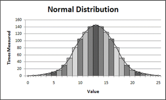 Figure 57. An example of a normal distribution.
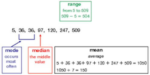 Figure 58. Illustrating the mode, median, mean and range in a data set. From Houghton Mifflin Math.
Data typically fit one of four scales: nominal, interval, ordinal or ratios. Of these data types, nominal and interval data are usually most important for rangeland monitoring.
A nominal scale assigns items to a group or category defined by one or more qualitative measures. Examples of these include: as grazed, ungrazed, lightly grazed, heavily grazed, or the length of the post-grazing recovery (growth) period (full season, most of the season, some chance, little chance or no chance). There are no numeric values or relationships among variables. The only applicable statistics are the frequency of occurrence and mode of the specific categories. When using the nominal scale, include or consider all possible responses, including the category “don’t know,” to prevent forcing answers into an inappropriate category. Also, all categories must be clearly defined so they are mutually exclusive of one another.
An interval scale is one where the distance between measures is always the same. Many different examples exist, including: year, percent cover or utilization, plant density, and stubble height. The key point is that the distance from one unit to the next is always the same.
An ordinal scale ranks members in order, but the magnitude of each member is not recorded. An example is the most dominant or abundant plant in a sample, second most, third most, etc. Such data for many samples could be used to determine if there has been a shift or if there is a difference in dominance between locations.
Ratios describe something in relation to something else, such as a plant root-to-shoot ratio or creek width to depth ratio. However, these are made out of interval scale data.
Analyzing Descriptive Data
Measures of central tendency (mean, median, mode) are single values used to characterize an entire set of data points (e.g., the average value from 50 quadrats used to measure bunchgrass density). The single value identifies the center of the distribution for each population. When two or more populations are sampled, investigators can calculate the central tendency of each and compare their values to one another through statistical calculations and tests.
The mode is applicable to both qualitative (descriptive) and quantitative (numeric) data. The mode represents the response or value that occurs most frequently. It is the easiest statistic to calculate because it is a simple count of the number of responses in each category; of each value; or of each range of values if interval data are divided into groups, such as low, middle and high. The mode is not affected by extreme responses or values, but can be unstable when the range of responses can have two or more values (sometimes widely spaced with other values in between) that are the mode. Although the mode identifies the most common response or score, it may not reflect the majority of responses or scores. It is the peak of the distribution curve. The most appropriate use of the mode is for nominal data.
The median is the midpoint in a range of scores and is applicable only to quantitative data. Half of the data points are above the median value and half below. When the number of data points is an even number, the median is the midpoint between the two middle scores. Every data set has only one median value, and that value is not influenced by extreme events; therefore, it is informative when interval data are not normally distributed, but skewed by very high or low values.
The mean is the arithmetic average of the data. It is the summation of the values for every data point, divided by the number of data points. It is applicable only to quantitative data, and there is only one mean value possible for each variable/attribute measured. Unlike median and mode, the mean is influenced by extreme values. It can be skewed far to the right or left of the median or mode. The mean is a very appropriate statistic for interval data such as biomass production, percent cover, density of plants, residual plant height and many other attributes.
It is often helpful to calculate more than one statistic for central tendency, particularly if data are not normally distributed. The use of two or more measures of central tendency often provides a more accurate interpretation. All measures of central tendency, however, must be interpreted with respect to sample size. Small sample sizes can provide misleading statistics, particularly if sample sites are not randomly selected, and/or the data have large variation.
All data sets have variation. The important question is how large or small is that variation. Full interpretation of the mean, median or mode for all data requires that the investigator understand the variability of the population’s responses. Interpretation may be quite different if the variation of the data around the mean is large compared to being very small. Common measurements of variation are the range, variance, standard deviation, confidence intervals, and the coefficient of variation, quartiles, skew and kurtosis.
The range is simply the difference between the highest and lowest recorded values. The degree of spread from the mean, median, or mode is an indicator of the variability (for the sampled attribute) of the population’s responses. These values, however, should be checked to determine if they are outliers from “most” responses. Unique high and low values are extreme compared to most responses may be meaningless as an indicator of the range of variability. An outlier reflects some factor unrelated to the population or communities response.
Variance and standard deviation measure the collective difference between the mean and individual data points. Specifically, variance is the average of the squared deviations from the mean. Squaring the difference between each data point and the mean makes all values positive, and dividing the sum of all of the squares by the number of data points avoids increasing the value with a larger sample size. Standard deviation is the square root of the variance.
In practical terms, the larger the variance or standard deviation, the greater the dispersion of the individual data points around the mean. That is, many data points are far from the mean value. A small variance or standard deviation indicates very similar responses or measurements, and most data points are near the mean.
 Figure 59. Graphs of negative and positive skew.
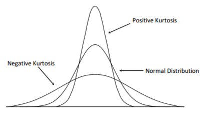 Figure 60. Graphs of negative and positive kurtosis.
The smaller the variance or standard deviation, the greater the probability that the mean obtained from the samples collected is close to actual value of the attribute being measured for the entire population. The terms large and small are relative and directly related to the scale of the data set. When the range of responses is from 1 to 5, a variance of 4 (standard deviation = 2) is very large. When the response range is from 1 to 100, a variance of 4 (standard deviation = 2) is quite small. From a practical perspective, when the mean for sagebrush cover is 16 percent and it has a variance of 0.50 percent, one can reasonably conclude the sagebrush cover is near 16 percent. If the variance were 5 percent, there would be a good probability the true sagebrush cover on the site could be much less or much greater than 16 percent.
The confidence interval is composed of two values, one on each side of the mean, that identify the range of values likely (given a specific probability level) to include the true mean for the population. The calculated mean of a sampled attribute is always the mean value for the data points (samples) collected, and is an estimate of the actual mean of the population. The actual (true) mean for the population is almost always different from the sample mean and can only be determined if every potential sample is measured (often infeasible). The confidence interval identifies specific values on both sides of the sample mean, and the true mean of the population is likely to fall within these two values, given a specified level of probability (e.g., 95 percent). For example, if the sample mean is 25 and the 95 percent confidence interval of the population mean ranges from 21 to 29, there is a 95 percent chance the true mean of the population is a value from 21 to 29. For a given sample mean, the higher the probability selected (99 versus 95 percent) the broader the confidence interval will be around the mean. Data with high variability have wider confidence intervals than data with low variability. Selecting an appropriate probability value (a function of the importance of the attribute) is important for calculating a confidence interval.
The coefficient of variation (CV) is expressed as a percent. It is a relative measure of variability. In contrast, the standard deviation is an absolute measure because it is measured in the same units as the observations. The larger the CV for an attribute, the greater the variability of the attribute sampled. Specifically, the CV is the sample standard deviation divided by the sample mean, multiplied by 100.
Quartiles may be the best indicator of variability when the data distribution is highly skewed. Quartiles are intervals that contain 25 percent of the data points. The width of the intervals is an expression of variability in the data. The width of the quartiles on either side of the mode may be small, but very wide toward the skewed tail. This pattern would indicate most of the population responded similarly, with some extreme outliers. If there are few outliers, it may be best to exclude them from data analysis and interpretation. For example, a sample can be divided into four (quartiles) or any other number of equal width (spread) intervals.
Skew describes how the distribution of the data points compared to the theoretical normal distribution, which is symmetrical. Variation from the normal distribution is skewness. Most data, typically, are skewed to some degree to the right or left of the mode, particularly if extreme values are present. When skewness is high, the assumption of normal distribution is not met, and the use of many parametric statistical tests, such as t-tests and analysis of variance, is not valid. The use of the mean to characterize the population may be a poor indicator of central tendency. Likewise the variance and standard deviation would be poor indicators of sample variation.
Non-parametric statistical tests (e.g., Wilcoxon Signed Rank Test, Kruskal-Wallis One-Way ANOVA) are more appropriate statistical tools when the assumptions required for proper application of parametric tests are not met.
Kurtosis reflects whether the distribution of data points or “curve” is peaked or flat. It identifies the steepness of the curve at the mode. Very steep curves indicate each data point has a similar value; thus, low variation. Very shallow (broad curves) indicate wide variation among the data points.
Surveying Populations
Sample Size
Land managers implementing a monitoring program must determine what proportion of the target population should be sampled to have enough statistical confidence that the data gathered adequately characterizes important ecological attributes (based on management objectives) in the management unit, and is likely to detect the effects of management actions. Most statistics textbooks offer a table for determining sample size.
Most monitoring studies do not test a research hypothesis; therefore, they lack (and do not require) the rigid experimental design required to detect small changes in ecological attributes with very high confidence (i.e., small p-values = small probability of thinking there is an actual difference when there is not). Rather, the quantity and perhaps the quality of the data and associated statistical analyses are explanatory studies, whose intent is to acquire adequate general information about baseline conditions and/or trends for important attributes and/or issues. There is a big difference between the statistical rigor (power) required to test a potential vaccine versus determining whether basal cover of perennial grasses has changed due to a management action. Large samples provide greater confidence that the summarized results accurately reflect the population; however, small samples can provide important information that may not be “statistically significant (i.e., small p-values of 0.05 or less)”, but may be “biologically significant,” or have management importance.
Sampling Methods
Specific sampling methods include simple random sampling, systematic sampling, stratified sampling and cluster sampling. With random sampling, every member (or all locations) in a given population (area) have an equal chance of being selected. Complete random sampling for questions that address large spatial areas typically requires more resources than are available for most rangeland monitoring programs. Random sampling may be appropriate for attributes measured on one (or only a few) small critical areas where one is looking for change across time at that location.
Systematic sampling typically places the entire population on a list, randomly selects one individual or starting point, and all subsequent sample units (quadrats, transects, plants, etc.) are equally spaced (e.g., quadrat placed every 5 feet on a transect).
Stratified sampling identifies certain subgroups in the population and samples each group in proportion to their numbers in the total population, or their degree of importance. The goal of stratification is to identify (separate) discrete entities (e.g., ecological sites) that are important, and collect the right number of samples from each entity of interest. This approach is intended to decrease variability by focusing only on the area, group or subpopulation of interest. This saves money (smaller sample sizes) and results in appropriate statistical power.
Cluster sampling does not target any individual as part of a sample, but rather includes a naturally occurring group, that occurs in a hierarchy. For example, sampling a stream in a watershed may occur at three levels: the watershed, specific reaches and channel units within a reach. Each of these groups forms a natural cluster. Within each cluster, samples are often obtained with either random or proportional sampling.
Sources of Sampling Error
There are several potential pitfalls that investigators must consider when sampling a population. Some of these include sampling and measurement error.
Sampling error - Sampling error occurs as a result of surveying only part of the population and results in statistics that differ substantially from actual value of the population. For example, basal cover of bunchgrasses for the sample obtained was 6.8 percent, but basal cover for the population is actually 5.1 percent. Sampling error is a function of sample size and is greatest when the sample is small and population variability large. The best method for overcoming sampling error is to increase sample size, or if appropriate stratify the management unit into appropriate sub-units that are more homogeneous. The sub-units must be relevant to the management goals and objectives. Management sub-units that are not relevant to identified management goals, objectives or issues may be excluded from having sampling sites.
Measurement error reflects variation in the data due to the lack of uniformity in the data collection process within and/or among sites. Measurement error often occurs due to poor definitions of the attributes being measured; inconsistent application of the monitoring protocol; the use of damaged sampling equipment; not locating or establishing sample units (transects, quadrats, etc.) with the same protocol at each location; collecting data in windy versus calm conditions; and any other factor that results in the same measurement of the same sampling unit being different, if the data were collected a second time.
Test Statistics and P-Values
When two sets of data are compared and statistically analyzed, the comparison is usually of their mean values (and their variation). The comparison often is for data from the same site collected in two or more years, or data collected from different locations in the same year (but across sites with some unifying feature and management objective). If the data comparison involves two samples (years or sites), the test statistic is a two sample t-test. When data from three or more samples (years or locations) are compared, the one-way analysis of variance is the best analytical tool. When the ANOVA suggests there is a high probability that one or more of the means differ from the others, a means separation test (e.g., Tukey or Least Significant Difference) can be used to show which means likely are different from one another.
Comparisons of means from different data collection periods (years) or locations (sites) will include a management hypothesis (also called null hypothesis in statistics books) and an alternative hypothesis. The management hypothesis typically states that the change in management has had no effect, correlation or association toward the attribute measured. For example, there is no difference in basal cover of desired perennial bunchgrasses five years after changing management from annual season-long grazing (i.e., growing season use every year) to rest-rotation grazing (periodic annual rest). The alternative management hypothesis may be stated as: five years after the implementation of rest-rotation grazing, there will be an increase in the basal cover of desired perennial bunchgrasses. The management question is: can the difference in mean basal cover of perennial bunchgrasses be confidently attributed to the change in grazing management, or is it likely due to some factor other than the change in management.
All statistical tests compute a p-value, which is presented in decimal format with a range from 0 to 1.0 (e.g., p = 0.10). The p-value is the probability of getting the results you obtained (or a more extreme difference between the mean values) given that the management (null) hypothesis is true (i.e., management had no effect on the means and they are similar). This probability reflects the evidence for or against the management hypothesis. The smaller the p-value (closer to zero), the greater the evidence (stronger confidence one has) against the management hypothesis (no difference due to management). The larger the p-value (closer to 1.0), the stronger the evidence for the management (null) hypothesis (no difference due to the treatments). P-values do not prove or disprove the management hypothesis (or the alternative hypothesis); they only provide strong to weak evidence (probability) for or against a hypothesis. Scientists who implement rigorous experiments often state that when a comparison of two or more means results in a p-value of 0.05 or less, the means are significantly different and they would reject the null/management hypothesis, and accept the alternative hypothesis. They typically conclude that if the test statistic had a p-value of 0.06 the means would not be significantly different from one another, and they would accept the null hypothesis. For land management, much larger p-values may be quite acceptable (e.g., p = 0.20 or 0.30) if the change has been consistent across monitoring sites and in a desired direction. Management looks for the preponderance of evidence, not conclusive evidence.
When samples are collected from either the same or different populations, the mean values will almost always be different. For example, basal cover of perennial grasses may be 8.24 percent in one sample and 8.31 percent five years later. The practical question is: is there a strong or weak probability (evidence) that the difference between the two means is due to the management applied to the site. The p-value provides evidence for or against the management hypothesis, but provides little if any information about the size of the effect of the management action. The size of the effect of a management action can be estimated with effect size statistics.
Effect Size Statistics
Effect size equations (statistics) report the magnitude and direction of the difference between two means. There is not a direct relationship between the size of a p-value and the magnitude of effect for a management action (Table 1). A small p-value (P<0.05) can occur with either a small or large management effect, as can large p-values. Monitoring studies often do not achieve small p-values for numerous reasons, and the cost of establishing enough monitoring sites and collecting large enough sample sizes to obtain very small p-values would prevent most if not all monitoring from occurring. P-values between 0.06 and 0.20 (or perhaps even larger) may lead to a conclusion that there is strong support for the management hypothesis. That is, there is sufficient evidence (i.e., high probability) to conclude that there is no difference in the means because of management actions. Management, however, can still have had an effect that may range from nearly nothing to very large, with either small and large p-values. Effect size statistics look at practical versus statistical significance.
The data below in Table 1. compares General Agriculture Perceptions by Students in Schools with an Agriculture Program versus Students in Schools with No Agriculture Program (N = 1,953). Traditional statistical analysis found a significant difference between the mean (p=0.046). Effect size analysis, however, found at best a very small effective difference (Cohen’s d) in perceptions about agriculture regardless of the type of school attended. This example illustrates the hazard of using only p-values to interpret data. This example is from Kotrlik et al. (2011).
Three effect size statistics can be used to analyze whether or not a change in management has resulted in a desired effect. Each uses standard descriptive statistics to measure effect size. The equations are based upon the mean difference for data collected between two sites or two dates, and that difference is divided by the standard deviation from the control site, or a pooled value from the standard deviations from both sites. Among the three equations Cohen’s d and Hedge’s g are most popular, with Hedge’s g providing a slightly better result for small sample sizes. One does not need to understand the equations for calculating the pooled standard deviation. Numerous internet-based sites can be used to calculate effect size using your mean and standard deviation data for any data set. To obtain effect size results you can use interactive calculators on the following sites: http://www.polyu.edu.hk/mm/effectsizefaqs/calculator/calculator.html and http://www.psychometrica.de/effect_size.html#cohen.
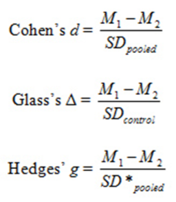 Figure 61. Three most common effect size equations.
The general guideline for interpreting the effect size statistic from the three aforementioned equations is as follows: no effect to a small effect when the effect size value ≤ 0.30; a moderate effect for effect values between 0.30 and 0.59; a large effect when the effect size ranges from 0.60 and 0.89, and a very large effect when effect size value ≥0.90. As with all guidelines, a question is, what are the practical interpretations of the data and the results of the statistical analyses. To address this question, it may be useful to compare the effect size obtained to the maximum possible or expected effect size effect given your understanding of the ecological relationships involved.
Table 1. Student perceptions in agriculture.
| Student Perceptions |
Agriculture Program
M |
Agriculture Program
SD |
No Agriculture Program
M |
No Agriculture Program
SD |
t |
df |
p-value |
Cohen's d |
| of Agriculture |
20.11 |
2.68 |
19.86 |
2.55 |
2.00 |
1767 |
0.046 |
0.10 |
Data Presentation
Summarized data should be presented in a logical and concise manner. This may include a combination of text, charts, tables, and graphs.
Text
Text increases clarity and provides an analysis/interpretation of the results. Text becomes important if there are other data that were not collected by the investigators of the current monitoring study, but which they use in the analysis of their results or to justify their conclusions or management recommendations. This is important because most of this appendix is about detecting change or differences. The concern is, whether a difference in the data was related to the management applied, or not. Short-term monitoring is essential for interpreting long-term trends, and context is essential for interpreting spatial differences.
Charts
Charts combine pictures, words and/or numbers that often show important trends and variation. Charts can graphically illustrate sequential steps much clearer, and often more concisely, than lengthy text. Charts delineate and organize complex ideas, procedures and lists of information.
Tables
Tables summarize large amounts of data and can illustrate differences between groups or populations. They report a numeric value for a category that can be qualitative (e.g., light utilization) or quantitative (e.g., percent cover). Tables group variables from data sets to illustrate comparisons. Table 2. below shows the variables measured across the top row and then the summary statistics for each variable underneath.
Table 2. Vegetation data (Davies et al. 2006).
| Statistic |
Sandberg
Bluegrass |
Tall
Perennial
grasses |
Annual
Grass |
Perennial
Forbs |
Annual
Forbs |
Total
Herbaceous |
| Mean |
5.4 |
12.2 |
0.6 |
4.1 |
0.6 |
22.9 |
| Median |
5.3 |
10.9 |
0.1 |
3.6 |
0.4 |
21.9 |
| Minimum |
0.0 |
4.5 |
0.0 |
0.0 |
trace |
5.9 |
| Maximum |
13.2 |
28.3 |
9.8 |
11.9 |
5.6 |
46.5 |
| Standard Error |
0.23 |
0.5 |
0.1 |
0.3 |
0.1 |
0.66 |
Graphs
Graphs can also present summarized quantitative data. They are excellent for describing changes, relationships and trends. Graphs often convey information much quicker and clearer than text. Graphs allow the reader to visually observe the results and interpret their meaning, without having to read and interpret lengthy text. Graphs are generally preferred over tables when a visual result enhances understanding about the magnitude of differences at one point in time, or trends in change across time. Tables are appropriate when the specific numbers are needed to convey critical interpretation of data.
Pie graphs and histograms are excellent graphics for showing frequency data, when data are available for two or more categories or populations. Pie graphs are best for qualitative categories given a limited number of categories and succinct category labels. The pie chart below depicts the means from the table above.
Line Graphs
line graphs are excellent for illustrating change across time. Bar graphs demonstrate differences between two attributes at specific points in time. Bar graphs can be simple (single comparisons) or complex (multiple comparisons), and can be structured horizontally or vertically. Each bar summarizes a quantitative attribute (total, mean, median) about one or more populations for a specific attribute or question.
Scatter Plots
Scatter plots display the relationship between two variables, on an x-y graph. When variables are tightly grouped together, usually in a linear (or curvilinear) pattern, they typically have a strong correlation. Wide scattering of the data points around the mean or median, or around a regression line, indicates high variability in the data and poor or weak relationships or trends. In Figure 65, the solid line (just above the value 8) is the regression line for the relationship between year and inches of precipitation. The nearly flat trajectory of the line suggests almost no change (trend) in water-year precipitation since the 1870s. Wide spacing between the line and many data points across the entire period of record demonstrate great variability in water-year precipitation among years.
Websites to Access Statistical Tools
Webpages to perform statistical calculations can be found at: http://statpages.info/index.html. This site provides access to many different websites that provide simple to complex statistical analysis, plot data, create charts and other graphics, etc. All of the calculations and statistical tests described in this appendix, except for effect size statistics, can be conducted at many of the websites found on this website. Web pages for effect size calculations and explanations of effect size statistics can be found at https://www.uccs.edu/lbecker/ and http://www.psychometrica.de/effect_size.html#cohen.
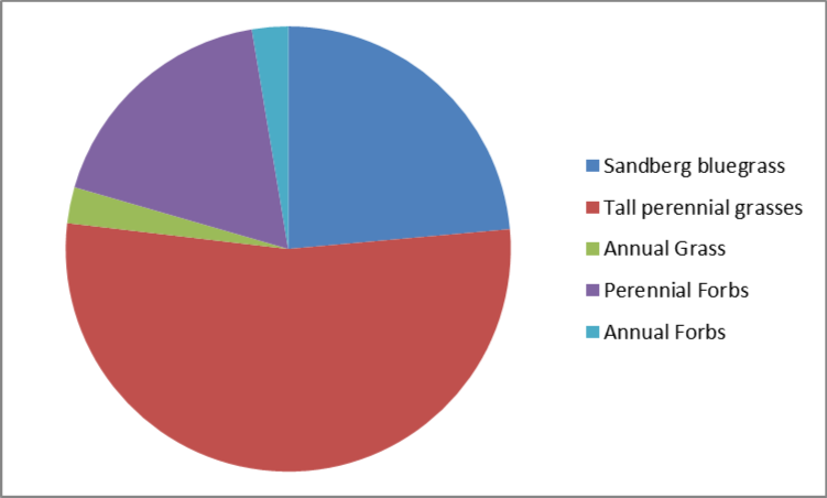 Figure 62. Vegetation data from Davies et al. (2006).
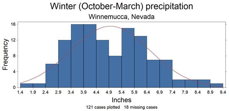 Figure 63. Histogram
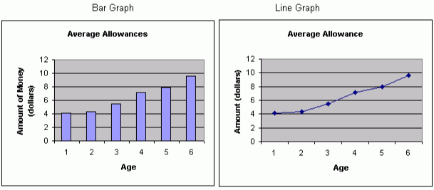 Figure 64. Bar graph and line graph.
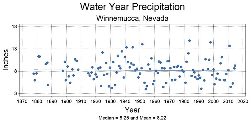 Figure 65. Scatter plot
Swanson, S., Schultz, B., Novak-Echenique, P., Dyer, K., McCuin, G., Linebaugh, J., Perryman, P., Tueller, P., Jenkins, R., Scherrer, B., Vogel, T., Voth, D., Freese, M., Shane, R., McGowan, K.
2018,
Nevada Rangeland Monitoring Handbook (3rd) || Appendix I - Statistical Considerations,
Extension | University of Nevada, Reno, SP-18-03