Evaluation Matters | 2026-10
In this edition
- A Tale of Two Candies
- Behind the Mask
- Harvesting Predictions
About Evaluation Matters
Evaluation Matters is a monthly newsletter published by the University of Nevada, Reno Extension. It is designed to support Extension personnel and community partners in building practical skills for evaluating programs, making sense of data, and improving outcomes. Each issue focuses on a key concept or method in evaluation and provides clear explanations, examples, and tools that can be applied to real-world programs.
This issue focuses on three ideas that help evaluators compare and predict with care: the logic behind comparing two groups, practical ways to protect participant confidentiality from data collection through reporting, and an introduction to simple linear regression.
A Tale of Two Candies
A short and sweet understanding of group comparison.
Which is bigger: a plain M&M or a peanut M&M? For most people, the answer seems obvious. Peanut M&M’s are larger. You probably did not need a ruler, a scale, or a statistical test to reach that conclusion. You have seen enough of both candies to know roughly what each one looks like, and the difference between them is large enough that the comparison feels easy. Without realizing it, however, you are already using some of the same logic that underlies statistical comparisons.
The important part is that no two M&M’s are exactly alike. Plain M&M’s vary slightly in size and weight, and peanut M&M’s vary even more because of the peanut inside each candy. One set of measurements found that peanut M&M’s weighed about 2.4 grams on average, but individual pieces ranged from roughly 1.5 to 3.5 grams. Plain M&M’s averaged about 0.9 grams and were more consistent from piece to piece (Weigh School, n.d.). Even with this variation, the difference between the two types is usually large enough that we have little difficulty telling them apart.
Now imagine that the candies were a little different. Suppose plain M&M’s came in a wider range of sizes. Some were tiny, some were large, and many were nearly the same size as peanut M&M’s. At the same time, imagine that peanut M&M’s had a larger variance from one candy to another. The average peanut M&M might still be larger than the average plain M&M, but the two groups would overlap much more. Suddenly, answering our original question would become more difficult.
This is where the logic of statistical group comparison begins. When we compare two groups, the difference between their averages is only part of the story. We also need to consider how much variation exists within each group. If the values within each group are tightly clustered, a relatively small difference between the averages may stand out clearly. If the values are spread widely, even a noticeable difference between the averages can become harder to interpret.
Imagine reaching into two bowls and selecting five candies from each. The five peanut M&M’s you grab might be unusually small, while the five plain M&M’s might be larger than usual. Looking only at those ten candies, you could get a misleading impression of the two groups. If you reached into the bowls again, you might select a different combination and see a somewhat different result. This is the challenge of working with samples. We rarely observe every person, program, classroom, county, or other member of the population we want to understand. Instead, we collect a sample and use it to learn something about the larger group.
Extension data work the same way. Suppose an Extension team compares post-program confidence scores across two counties offering the same type of nutrition education program. Participants in one county report an average confidence score of 4.2, while participants in the other average 4.6. The second county has the higher average, but that alone does not tell us whether the difference is meaningful. If nearly everyone in the first county scores between 4.1 and 4.3 and nearly everyone in the second scores between 4.5 and 4.7, the separation between the groups is fairly clear. If scores in both counties are spread widely between 2 and 5, the difference between the averages is small compared with how much participants differ from one another.
Statistical comparison tests help us evaluate these pieces together. Tests that compare group means consider the difference between the sample averages relative to its standard error. That standard error reflects both the variability within each group and the number of observations collected. With sample sizes held constant, greater variability generally makes a mean difference harder to estimate precisely. The underlying question is whether the pattern we observed is strong enough to stand out from the ordinary variation we would expect when sampling people from a population.
This basic concept sits underneath many statistical tests. A two-sample t-test compares two group averages, while analysis of variance, or ANOVA, extends the same general logic to three or more groups. Other methods address different types of questions and data, but much of inferential statistics begins with the same challenge: separating patterns that appear meaningful from differences that might reasonably occur through ordinary sampling variation.
So, did you know that you were performing a statistical comparison when differentiating between M&M types? You didn’t calculate a mean, standard deviation, or p-value, but your brain was still weighing the same basic pieces of information. Peanut M&M’s are larger than plain M&M’s, and the variation within each type is small enough that the difference is easy to recognize. Statistical tests formalize that same reasoning when the answer is less obvious. In that sense, a handful of Halloween candy offers a pretty good introduction to the logic behind group comparison.
References
Weigh School. (n.d.). M&M weights and calories (in pictures & charts). https://weighschool.com/mm-weights-and-calories/

Comparing two groups means looking at the variation within each group as well as the difference between their averages.

Top row: plain (left) and peanut (right) candies with little variation. Bottom row: the same two types with wide variation.
Behind the Mask
Practical ways to de-identify data, store it, and report small groups thoughtfully.
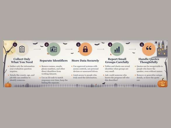
Halloween is a season of masks, disguises, and hidden identities. In evaluation, keeping an identity hidden can be important for a very different reason. Participants often share information with the expectation that their individual responses will remain private, particularly when surveys, interviews, or focus groups ask about personal experiences, opinions, or challenges. Protecting that confidentiality requires more than simply removing a person’s name from a spreadsheet. Other details in the data can sometimes make an individual surprisingly easy to identify. Evaluators can protect their records and their own reporting, but they cannot guarantee that other focus group participants will keep what they hear private.
One of the simplest ways to protect confidentiality is to collect only the information you actually need. Every additional piece of identifying information creates another opportunity for someone to be recognized. If your evaluation question does not require a participant’s full name, home address, exact birth date, or other identifying detail, there may be little reason to collect it. Even information that seems harmless on its own can become identifying when combined with other variables. A person’s county, age, job title, and program role, for example, might describe only one individual in a small program.
Removing direct identifiers is an important first step. Names, email addresses, phone numbers, identification numbers, and other obvious identifiers should usually be separated from the dataset used for analysis. If participants need to be matched across multiple surveys or time points, an identification code can often be used instead, essentially giving each participant a mask within the working dataset. A separate file can connect that code to the participant’s identity when necessary, while the working dataset contains only the code. Keeping those files separate limits the number of places where identifying information appears.
Secure storage is another important part of confidentiality. Evaluation data should be kept in approved systems with appropriate access controls rather than on personal devices, unsecured drives, or unrestricted shared folders. Access to shared folders should generally be limited to the people who actually need the information to complete the evaluation, and thoughtful file permissions can prevent accidental disclosure while still allowing the team to collaborate effectively.
Confidentiality also matters after the analysis is complete. Tables and charts can reveal identities even when they do not contain names. Imagine reporting results from a county program in which only three participants are over the age of 70. A table showing that all three selected the same response may effectively reveal how each person answered, particularly to staff who know the participants. The same problem can occur when results are divided by race, occupation, community, program site, or another characteristic that produces very small groups. Before sharing a table or chart, ask whether someone familiar with the program could reasonably determine who the data describes.
Qualitative information deserves the same attention. A quote may be presented without a name but still be recognizable to people who know the speaker. A participant might mention a unique job, describe a highly specific experience, name a location, or refer to an event that only a few people attended. Removing the person’s name does not necessarily make the quote confidential. In some cases, small details can be removed or generalized while preserving the meaning of the comment. In others, the safest decision may be to not use the quote at all.
This could be especially relevant in small communities, where people may know one another well and individual experiences can be easier to recognize. A statement such as “a participant in a rural county” may sound anonymous, but adding age, occupation, program role, and a distinctive quote could narrow the possibilities quickly. Evaluators should think about confidentiality from the perspective of someone who already knows the community. The question is not only, “Did I remove the name?” but also, “Could someone reasonably figure out who this is from everything else I provided?”
A useful practice is to conduct a confidentiality review before results are shared. Look through tables for very small groups, scan quotes for identifying details, and consider whether combinations of variables could reveal an individual. Check who has access to the underlying files and whether identifying information is stored separately from analysis data. These steps do not require sophisticated technology, but they can prevent problems that are difficult to fix after a report, presentation, or dataset has already been distributed.
Protecting confidentiality ultimately comes down to being intentional about what we collect, where we keep it, who can see it, and how we share it. By collecting only necessary information, limiting access, separating identifiers, and reviewing results carefully before publication, evaluators can reduce the chance that participants will be recognized. In evaluation, the goal is not to hide the data, but to mask the details that could reveal who provided it.
Harvesting Predictions
A brief introduction to simple linear regression. The line, the intercept, and what does residual mean?
You may remember the equation y = mx + b from algebra. The letter m represents the slope, or how much y changes when x increases by one, while b represents the intercept, where the line crosses the vertical axis. If the equation is y = 0.5x + 1, an x value of two produces a y value of two, an x value of four produces three, and an x value of six produces four. Plot those points, and they fall neatly along a straight line (Figure 1, left). Once we know the equation, finding another point is simply a matter of plugging in a new value of x.
Real-world data are rarely that tidy. Imagine plotting a set of observations and finding that the points generally rise from left to right, but they do not sit perfectly on a single line. Some points are above the pattern, others are below it, and no simple equation describes every observation exactly (Figure 1, right). We could draw many different lines through those points, but some would represent the overall pattern better than others. Simple linear regression turns the algebra problem around: instead of starting with an equation and finding the points, we start with the points and estimate the equation that best describes them.
That estimated equation still takes a familiar form. Suppose an Extension gardening program examines the relationship between the number of training hours participants complete and their final knowledge scores (Figure 2). Training hours become x, while knowledge score becomes y. If the fitted regression equation were predicted knowledge score = 50 + 4(training hours), the model would predict a score of 70 for someone completing five hours of training. The equation gives us a way to estimate an outcome from a value we already know.
The slope tells us how the predicted outcome changes as x changes. In this example, the slope is four, meaning each additional hour of training is associated with a four-point increase in the predicted knowledge score. A participant completing six hours would therefore have a predicted score four points higher than someone completing five hours. Importantly, this describes the pattern in the data rather than proving that the additional hour caused the higher score. Participants who attend more training may differ in other ways that also influence their knowledge.
The intercept is the predicted value of y when x equals zero. In our example, the intercept is 50, so the regression line crosses the knowledge-score axis at 50 when training hours equal zero. Sometimes that number has a useful interpretation, but not always. If everyone in the dataset completed at least two hours of training, we do not actually have information about participants with zero hours. In that case, the intercept helps position the line mathematically without necessarily telling us something meaningful about the program.
Of course, the actual observations will not all land exactly on that line. A participant who completed five hours might earn a score of 76 even though the model predicted 70. The six-point difference between the observed score and the predicted score is called a residual. Some residuals will be positive and others negative, depending on whether a point falls above or below the line (Figure 3). Ordinary least-squares regression finds the line that minimizes the sum of the squared residuals, the squared differences between observed and fitted values. A residual is the observed value minus the fitted value.
Another number commonly reported with regression is R², pronounced “R-squared.” R² describes how much of the variation in the outcome is accounted for by the regression model. If R² equals .40, the model accounts for 40% of the observed variation in knowledge scores. That does not mean the model correctly predicts 40% of participants, nor does it mean training hours caused 40% of the variation in their scores. It simply tells us how closely the line captures the overall pattern in the data.
A regression line can also be used to make predictions, but those predictions need to stay grounded in the data used to create the model. If participants in our program completed between two and ten hours of training, using the equation to predict what would happen after 20 hours would extend far beyond the information we actually observed. Relationships can change, level off, or behave differently outside the range of the original data. Looking at the scatterplot alongside the regression results helps us see whether a straight line is a reasonable summary in the first place.
Simple linear regression builds on a familiar idea from algebra but adapts it to the messiness of real data. The slope describes the direction and amount of change in the predicted outcome, the intercept positions the line, residuals show how individual observations differ from their predictions, and R² describes how much variation the model captures. Together, these pieces allow evaluators to move beyond simply noticing that two variables are related and begin estimating how one changes alongside the other. The points may not fall perfectly on the line, but regression gives us a useful way to describe the pattern they create.

A regression line describes how a predicted outcome changes as the predictor changes.
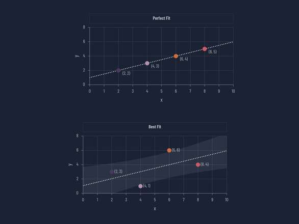
Figure 1. Top: points that fall exactly on a straight line. Bottom: points that scatter around the line that best fits them.
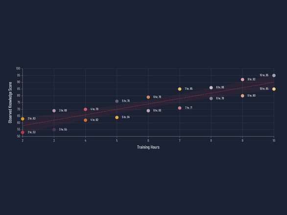
Figure 2. Observed knowledge scores at each number of training hours in the gardening example, with the estimated regression line.
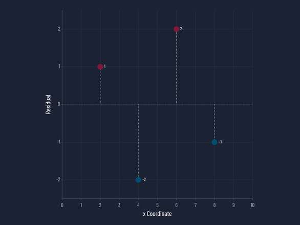
Figure 3. Residuals from the best-fit line in Figure 1: each point’s vertical distance above or below that line.
Published by:
Copp, C. & Elgeberi, N., 2026, Evaluation Matters | 2026-10, Extension, University of Nevada, Reno, Newsletter
An EEO/AA Institution. Copyright © 2026, University of Nevada Cooperative Extension.
A partnership of Nevada counties; University of Nevada, Reno; and the U.S. Department of Agriculture
