Getting started with climate change planning: 
understanding and using climate projections

More and more communities are planning for climate change, but it can be hard to know where to start. This document answers some common questions about using future climate scenarios from global climate models and provides tips about how to choose climate projections and links to reliable sources of climate projections for Nevada.

What are global climate models?

Global Climate Models (GCMs) simulate how the Earth system changes under different conditions, such as varying levels of greenhouse gas emissions (GHGs). They are currently the best tool for examining potential future climates. Global Climate Models are mathematical models of the Earth system that simulate complex interactions among the atmosphere, oceans, land surface, glaciers and sea ice. Some models also simulate how the global biosphere influences climate. In addition to simulating climate conditions for the future, the same models simulate climate conditions for the past using observations of solar radiation, volcanic eruptions, greenhouse gas and aerosol emissions, and land use. These historical simulations can be compared to observations to determine how well the model represents past climate. Some models do a better job of representing some parts of the climate system than others. There are over 30 GCMs used to project how climate may evolve through time. All of these models are run under an agreed upon set of future emissions scenarios to compare climates simulated by the models and present a range of future outcomes. 

Why do climate projections differ?

Parameterization is a way of simplifying the math used to model complex earth processes. Parameterizations are used when physical processes, such as cloud formation, occur at smaller scales than the grid boxes and cannot be properly modelled. Different GCMs have unique parametrizations. This is often referred to as model uncertainty.

External forcing refers to different factors that affect the Earth’s climate and “force” or cause the climate system to change. External forcings include solar variations, volcanic eruptions, greenhouse gas emissions and aerosols. This is often referred to as scenario uncertainty because they are described by the emissions scenarios.

Natural climate variability refers to differences from internal interactions of the climate system. Climate oscillations that affect natural variability include features, such as El Niño and La Niña and the Pacific Decadal Oscillation. These occur in the models but not necessarily at the same time (e.g., a La Niña year in one model could be an El Niño year in another). This is often referred to as internal variability uncertainty. 

Uncertainty in how much climate will change by the end of the century is dominated by scenario uncertainty—how people globally address rising GHG concentrations in the atmosphere. Model and internal variability uncertainty are more important over the next few decades and over smaller regions.

Coupled Model Intercomparison Projects (CMIP) scenarios 

The World Climate Research Programme organizes the Coupled Model Intercomparison Projects (CMIP) to better understand how past climate varied and how climate might change in the future, given different emissions scenarios. These are done partly to support Intergovernmental Panel on Climate Change (IPCC) Assessment Reports. Each CMIP project uses agreed upon scenarios with different levels of GHG emissions. The most recent is CMIP6 which uses Shared Socio-economic Pathways (SSPs). The previous one, CMIP5, which was used in the 2013 IPCC Fifth Assessment Report and the 4th National Climate Assessment, used Representative Concentration Pathways (RCPs). As of 2022, CMIP6 is still new, so most easily accessible regional climate projection data is from CMIP5. New CMIP6 data will become available more widely accessible in the coming years. 

Technically, neither SSPs or RCPs describe specific levels of GHG emissions. Instead, they outline radiative forcings. Radiative forcing describes how much more energy is available to the atmosphere. Higher emissions cause higher radiative forcing and higher global temperatures, and it’s common to see plots showing the GHG emissions needed to produce a given radiative forcing scenario (Figure 1). Often people refer to the RCPs and SSPs as emissions scenarios.

In addition to describing the radiative forcing, SSPs include descriptions about how the world will change and what steps we take to mitigate climate change. 

More recently, warming levels have been used instead of scenarios. A warming level uses all the scenarios that reach a global level of warming, such as 1.5 C or 2 C higher than pre-industrial (1850-1900) temperatures. This can make it easier to compare some regional impacts but complicates assessing variables like sea-level rise that respond slowly.

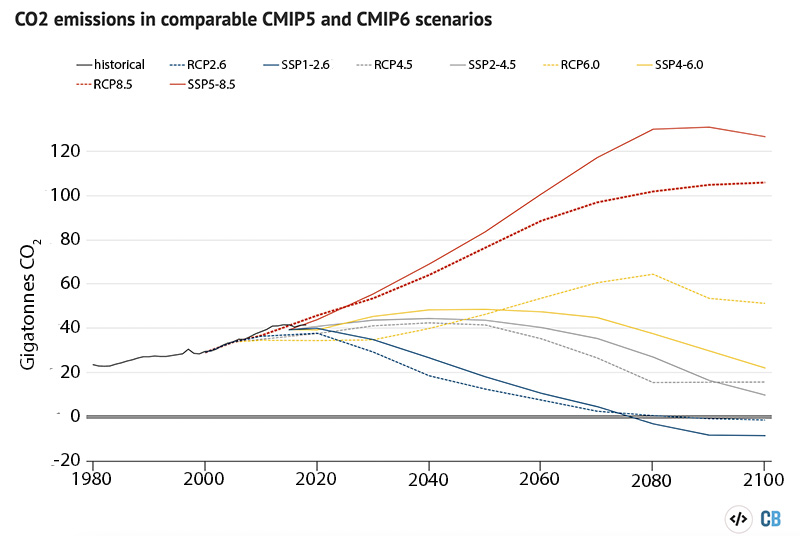
Figure 1. This image from CarbonBrief (https://www.carbonbrief.org/cmip6-the-next-generation-of-climate-models-explained/) compares greenhouse gas emissions in CMIP6 scenarios (SSPs, solid lines) to greenhouse gas emissions in CMIP5 scenarios (RCPs, dashed lines). Reproduced under CarbonBrief’s CC License. 

What is bias correction and why is it used?

GCM runs over the historical period are not meant to model the day-to-day weather that occurred. They are meant to simulate the climate, the long-term averages of variables such as temperature and precipitation, the usual amount of year-to-year variability, and the trends in climate. For example, the historical runs from GCMs may not have a major storm event in Reno in January 1997. However, the historical runs should display major features of the local climate. So, historical GCM runs should show that in northern Nevada, winters are wetter than summers. 
Because climate models are models, they do have some biases – or differences from observations. GCM variables can be corrected to better match the climate. This can be important if GCM projections are being used to track changes that require a very accurate baseline climate. One example of this is snow. If a model is too warm, too little of the precipitation will fall as snow, but if a model is too cold, the snow season might be too long. So, if in the historical run, the winter minimum temperatures are 5 F too high on average, and the summer maximum temperatures are too low by 3 F, the GCMs temperature data will be corrected by those amounts in both historical and the future runs. Bias correction approaches are continually advancing, and different kinds of bias correction may be suitable for different variables, time steps (e.g., daily or monthly), and average conditions versus extremes such as heat waves or severe storms.  

What is downscaling and why is it used?

The spatial resolution of GCMs (the size of the grid cells in the model) varies among models, but it is on the order of 100 km, or about 60 to 65 miles. This is too coarse to capture the diverse topography of Nevada. For example, Harry Reid International Airport (at 2,181 feet elevation) and Mt. Charleston (at 11,916 feet elevation) are about 40 miles apart. In a GCM, they could be in the same grid cell (Figure 2) and would have the same temperatures. In the real world, however, Mt. Charleston is typically much cooler (the annual average temperature is 47 F at the Mt. Charleston Ranger Station) than the airport (70.1 F). Because of this, models are downscaled, meaning various methods are used to add detail from observations or higher resolution models. Downscaling can produce climate projections with spatial resolutions as fine as 3 to 6 km (2 to 4 miles).

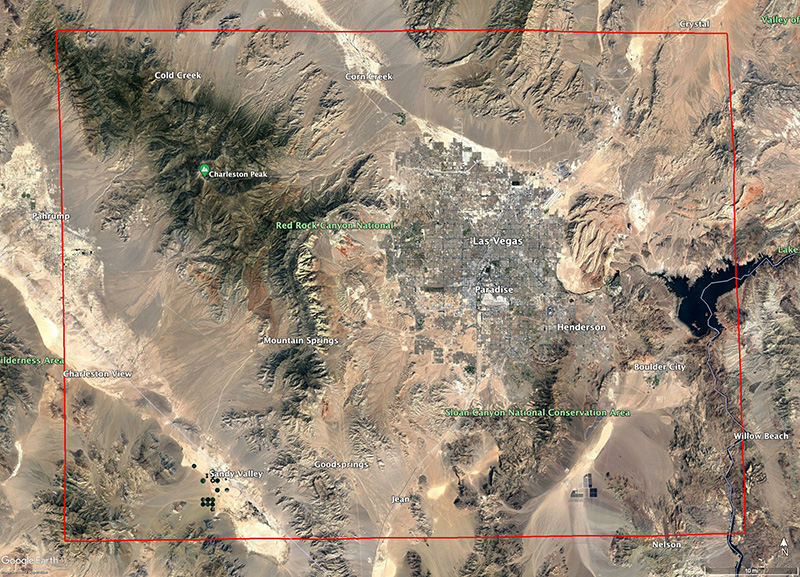
Figure 2. This image shows a 100 kilometer x 100 kilometer (62 miles x 62 miles) grid box over the Las Vegas metro area. Image from Google Earth.

There are two main kinds of downscaling.
Dynamical downscaling uses high-resolution climate or weather models to simulate local-scale atmospheric processes given the large-scale climate circulation in the GCM output. Dynamical downscaling produces a wide range of climate variables, often for multiple times throughout the day, and it can be used to study how fine-scale climate processes will change. However, it requires significant computer resources, so there are often fewer scenarios to choose from, a smaller set of GCMs and/or fewer emissions scenarios. The process of dynamically downscaling can also introduce new biases that differ from the GCMs.

Statistical downscaling uses statistical relationships between large-scale climate patterns in the GCMs and observed local climate. It can range from very simple techniques such as simply adding projected changes in temperature to existing climate data, or can be more complex, relating surface weather to circulation patterns in the atmosphere. Statistical downscaling requires less computing resources, so it is often used to downscale a larger number of future climates (more GCMs and/or future scenarios), and it can be used to produce finer spatial resolution data over large areas. However, the spatial resolution, variables downscaled and time step are limited to what’s available in observed data. As a result, statically downscaled projections are typically available for fewer variables, often temperature and precipitation, at daily or monthly time steps.

Using climate projections to assess climate vulnerability and plan for future climate

Climate projections provide a wealth of information for assessing vulnerability to climate change and adaptation planning. However, careful consideration is important to ensure that results answer the intended questions. Below is some general guidance on how to use climate models. 

Compare future GCM simulations to the same GCM’s historical run

Because each model is unique and has its own characteristics (even after bias correction), the best way to understand what the model is projecting is to compare the future years with the historical simulations from the same model. Sometimes researchers make multiple historical runs of the same GCM, so it’s important to ensure that the future projection is compared to the historical run it starts from. In most cases, the researchers producing downscaled and bias-corrected information or developers of tools using climate projections will have accounted for this already.

Always consider multiple GCMs 

Although there are some indications that certain models are better than others based on how well they simulate historical climate, no single GCM should be considered the “right” model for future change. Using more than one model will ensure that a range of future climates are included. At minimum, four GCMs should be used. More GCMs provide a broader view of the future, and it can help to use additional models, if resources allow.

Extremes pose the greatest climate hazards and should be part of any climate assessment

Extreme heat, drought, major storms, floods and extreme fire weather will have the most significant impact on any region. Assessing the frequency and intensity of these extremes in future climate is important in any climate vulnerability assessment and/or adaptation plan.

Averaging multiple projections minimizes natural climate variability

GCMs include natural variability, such as El Niño and La Niña. In GCMs, these events will happen in different model years, so averaging models together highlights changes that are due to GHGs and other forcings. This is called an ensemble. The more models that are included in the ensemble and averaged together, the less the impact of natural variability (Figure 3). However, averaging models together can be misleading if different models project different directions of change (Figure 4), and it will make extremes less extreme. 

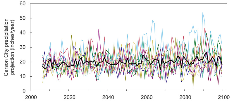
Figure 3. This plot shows the annual precipitation for Carson City projected by 10 climate models (thin colored lines) under the RCP8.5 scenario and their average in the thick black line. There is much more year-to-year variability in the individual models than in their average, and the very wettest or driest years are not the same in each model. Data from Cal-Adapt

Show the range of possible futures, not just the average change

This is especially important for precipitation. Over much of Nevada, averages show that precipitation will increase in the future, but the range often spans from a small decrease in precipitation to a large increase. For example, under the RCP8.5 scenario, the 20-GCM average shows that Elko will get wetter in both the winter and the summer. Twelve models do show that precipitation will increase in both seasons, but one model projects drier winters and wetter summers, five models project wetter winters but drier summers, and two models project that it will be drier in both seasons (Figure 4). 

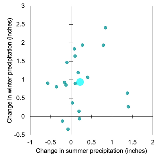
Figure 4. This shows the changes in winter and summer precipitation in Elko by the end of this century simulated under RCP 8.5 by 20 GCMs (small green dots) and the average change (large cyan dot). Data from ClimateToolbox.

A single gridcell from a GCM will differ from observations from a station within the gridcell

Measurements at a station generally will differ from the value in the enclosing gridcell. This can happen because the station has a different elevation from the gridcell average, or because of local influences by factors that are not resolved by the gridded data, such as hills, trees, clusters of buildings, etc. Because of this, it can be important to use some sort of bias correction to make the monthly mean of the gridded downscaled data match the station’s observed monthly mean. 

Whether or not to include multiple scenarios depends on how far into the future the assessment extends and what the goal is

The radiative forcings of different future scenarios are fairly similar to each other through about 2040 (Figure 5), so the climate changes also are often fairly similar. By the end of this century, some scenarios are for a much greater radiative forcing than others, so the climates can be quite different. If the goal is to describe climate at the end of this century for adaptation planning purposes, it is most helpful to use moderate and high-radiative forcing scenarios. In many cases, a reasonable place to start is to identify four “bracketing” scenarios that define futures that are (1) hot and relatively dry, (2) hot and relatively wet, (3) not as hot and relatively dry, and (4) not as hot and relatively wet. 

Figure 5. This shows summer (June - August) high temperature from 6 CMIP5 GCMs over Clark County. The grey is the historical period, with the green dashed lines showing observations. The red is a high scenario, and blue is a low scenario, with shading representing the range across models, and the bold line representing the mean. The two scenarios begin to separate around 2040.

In recent years, researchers have debated whether the level of emissions associated with RCP8.5 are likely. Some studies point out that recent emissions are lower than in RCP8.5 and that, with a shift from coal to other energy sources, emissions are likely to be lower than expected in RCP8.5. Other researchers note that changes in land use or ecosystem processes can also contribute to greenhouse gas emissions. Those changes are much more difficult to predict or quantify and could push us toward a future with very high emissions. With our current understanding, RCP8.5 might best be considered a reasonable but not inevitable “worst case” future that, in most cases, is useful as one of a set of scenarios. It can also be used alone if the goal is to focus on worst-case challenges.

Where can I find more resources about climate adaptation planning? 

Cal-Adapt (https://cal-adapt.org/) provides historical climate data and climate change projections for California and Nevada. There are many tools, but unfortunately, not all of them provide information for Nevada.

The Climate Toolbox (https://climatetoolbox.org/) has many easy-to-use tools for accessing current weather and climate information, forecasts over the next season, and future climate projections. Currently, the Climate Toolbox provides CMIP5 information for the lower 48 states.

The Aspen Global Change Institute’s User Guide to Climate Change Portals (https://www.agci.org/projects/climate-portal-guide) has in-depth information about the topics covered here and other sources of information.

Shared Socioeconomic Pathways 

Shared Socioeconomic Pathways (SSPs) are scenarios associated with different levels of radiative forcing and societal changes that affect emission levels. They’re used in CMIP6.

SSP1 - Sustainability

The world shifts towards renewable energy resources, lower consumption and sustainable infrastructure. This is the best case scenario in terms of keeping emissions low and climate changes small.

SSP2 - Middle of the road

The world makes some modest changes aimed at reducing emissions and adapting to climate change, but some efforts are more successful than others, so emissions remain moderate. This is a status quo scenario.

SSP3 - Regional rivalry

Sustainable development is a low priority in most parts of the world, because conflicts force countries to focus on local energy and security issues. There is some progress in keeping emissions relatively low, but it is largely because of poor economic conditions.

SSP4 - Inequality

Environmental progress is largely focused on local issues in richer nations, as inequalities around the world force developing countries to address conflict and unrest, hunger  and extreme poverty. Low-carbon energy sources are gaining popularity, especially in wealthier regions, but dependence on fossil fuels is still high where resources are less. Overall emissions are relatively low, in part because coal use drops.

SSP5 - Fossil-fueled development 

Innovation, technological progress and economic growth are placed at the forefront of sustainable development, but this advancement relies heavily on investment in fossil fuel resources. Progress is being made in health and education as the global economy grows, but these advancements come at the cost of very high greenhouse gas emissions.

Representative Concentration Pathways 

Representative Concentration Pathways (RCPs) specify the radiative forcing without describing the societal priorities that drive them. They’re used in CMIP5.

RCP8.5 - Rising radiative forcing

This scenario has very high levels of greenhouse gas emissions. It is likely if there is low effort to curb emissions, fossil-fuel energy remains dominant, and little societal progress is made towards more sustainable lifestyles. Environmental consequences are extremely high in this scenario, with high global average temperature increase, high sea level rise, and more extreme weather events. 

RCP6.0 - Stabilization without overshoot 

Under this scenario emissions rise until about 2060 and then drop, stabilizing at medium-high levels. This pathway is likely to result in slightly more modest levels of climate change than RCP8.5, but environmental consequences are still high in this scenario.

RCP4.5 - Stabilization without overshoot

In this medium-low emissions scenario, emissions inch up until about the middle of this century and then drop rapidly. It will probably require renewable energy use to become more widespread and lifestyles to shift to become less carbon intensive. This pathway is likely to result in moderate environmental consequences. Global average temperature, sea levels and the number of extreme weather events will still rise.

RCP2.6 – Reducing radiative forcing

In the event that there is a serious effort to curb emissions worldwide by shifting to dominant use of renewable energy, alongside developing innovative technologies, emissions could start dropping to very low levels this decade. Global average temperature rise would be kept to a minimum. This pathway could result in minimal environmental consequences compared to other scenarios.

Glossary

Earth system is the interacting physical, chemical, biological and geological processes on Earth. The system consists of the land, oceans, atmosphere and ice and the organisms that live in or on them.

Coupled Model Intercomparison Project (CMIP) is a collaborative framework organized by the World Climate Research Programme to advance climate change understanding by developing a set of standards and model experiments enabling comparison across climate models. 

Climate projections are simulations of the climate under a specific set of conditions, such as an emissions scenario.

Historical period is a set period of time when there are observations available and is often used to evaluate Global Climate Model performance. 

Emission scenarios are a set of projected changes in Earth’s energy budget related to greenhouse gas concentrations. As part of the CMIP project, GCMs from different institutions use the same scenarios as input to the model to project climate under these possible future scenarios.  

Radiative forcing is what happens when the amount of energy that enters the Earth’s atmosphere is different from the amount of energy that leaves it. If more radiation is entering Earth than leaving, as is happening today, then the atmosphere will warm.

References

• Abatzoglou, J. T., & Brown, T. J. (2012). A comparison of statistical downscaling methods suited for wildfire applications. International journal of climatology, 32(5), 772-780.
• Brekke, L. D., Miller, N.  L., Bashford, K. E., Quinn, N. W., & Dracup, J. A. (2004). Climate change impacts uncertainty for water resources in the San Joaquin river basin, California 1. JAWRA Journal of the American Water Resources Association, 40(1), 149-164.
• Burgess, M. G., Pielke, Jr. R., Ritchie, J. (2022). Catastrophic climate risks should be neither understated nor overstated. roceedings of the National Academy of Sciences, 119, e2214347119.
• Deser, C., Knutti, R., Solomon, S., & Phillips, A. S. (2012). Communication of the role of natural variability in future North American climate. Nature Climate Change, 2(11), 775-779.
• Flato, G., Marotzke, J., Abiodun, B., Braconnot, P., Chou, S. C., et al. (2013). Evaluation of Climate Models. In: Climate Change 2013: The Physical Science Basis. Contribution of Working Group I to the Fifth Assessment Report of the Intergovernmental Panel on Climate Change Cambridge University Press, Cambridge, United Kingdom and New York, NY, USA.
• Hausfather, Z. and Peters, G. P. (2020). RCP8.5 is a problematic scenario for near-term emissions. Proceedings of the National Academy of Sciences, 117, 27791-27792. 
• Hawkins, E., & Sutton, R. (2009). The potential to narrow uncertainty in regional climate predictions. Bulletin of the American Meteorological Society, 90(8), 1095-1108.
• Hayhoe, K., Edmonds, J., Kopp, R. E., LeGrande, A. N., Sanderson, B. M., Wehner, M. F., & Wuebbles, D. J. (2017). Climate models, scenarios, and projections. In: Climate Science Special Report: Fourth National Climate Assessment, Volume I [Wuebbles, D. J., Fahey, D. W., Hibbard, K. A., Dokken, D. J., Stewart, B. C., & Maycock, T. K. (eds.)]. U.S. Global Change Research Program, Washington, DC, USA, pp. 133-160.
• Riahi, K., Van Vuuren, D. P., Kriegler, E., Edmonds, J., O’Neill, B. C., et al. (2017). The shared socioeconomic pathways and their energy, land use, and greenhouse gas emissions implications: an overview. Global environmental change, 42, 153-168.
• Runyon, A. N., Carlson, A. R., Gross, J., et al. (2020). Repeatable approaches to work with scientific uncertainty and advance climate change adaptation in US national parks. Park Steward Forum 36. 
• Sanderson, B. M. & Wehner, M.F. (2017). Model weighting strategy. In: Climate Science Special Report: Fourth National Climate Assessment, Volume I [Wuebbles, D. J., Fahey, D. W., Hibbard, K. A., Dokken, D. J., Stewart, B. C., & Maycock, T. K. (eds.)]. U.S. Global Change Research Program, Washington, DC, USA, pp. 436-442.
• Schwalm, C. R., Glendon, S., Duffy, P. B. (2020). Reply to Hausfather and Peters: RCP8.5 is neither problematic or misleading. roceedings of the National Academy of Sciences, 117, 27793-27794. 
• Tebaldi, C., Ranasinghe, R., Vousdoukas, M., Rasmussen, D. J., Vega-Westhoff, B., et al. (2021). Extreme sea levels at different global warming levels. Nature Climate Change, 11(9), 746-751.
• USGCRP (2017). Climate Science Special Report: Fourth National Climate Assessment, Volume I [Wuebbles, D. J., Fahey, D. W., Hibbard, K. A., Dokken, D. J., Stewart, B. C., & Maycock, T. K. (eds.)]. U.S. Global Change
  Research Program, Washington, DC, USA, 470 pp., https://science2017.globalchange.gov/.
• Van Vuuren, D. P., Edmonds, J., Kainuma, M., Riahi, K., Thomson, A., et al. (2011). The representative concentration pathways: an overview. Climatic change, 109(1), 5-31.

All rights reserved. No part of this publication may be reproduced, modified, published, transmitted, used, displayed, stored in a retrieval system, or transmitted in any form or by any means electronic, mechanical, photocopy, recording or otherwise without the prior written permission of the publisher and authoring agency.
A partnership of Nevada counties; University of Nevada, Reno; and the U.S. Department of Agriculture